【Python计算机视觉编程】第二章 SIFT特征提取与检索及RANSAC实例
一.SIFT描述子
1.SIFT特征简介
1.1 SIFT算法可以解决的问题
(1) 目标的旋转、缩放、平移(RST)
(2) 图像仿射/投影变换(视点viewpoint)
(3) 弱光照影响(illumination)
(4) 部分目标遮挡(occlusion)
(5) 杂物场景(clutter)
(6) 噪声
1.2 SIFT算法实现步骤
SIFT算法的实质可以归为在不同尺度空间上查找特征点(关键点)的问题。
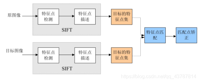
实现特征匹配流程如下:
(1) 提取关键点;
(2) 对关键点附加 详细的信息(局部特征),即描述符;
(3) 通过特征点(附带上特征向量的关 键点)的两两比较找出相互匹配的若干对特征点,建立景物间的对应关系。
1.3 关键点检测相关概念
这些点是一些十分突出的点不会因光照、尺度、旋转等因素的改变而消失,比如角点、边缘点、暗区域的亮点以及亮区域的暗点。既然两幅图像中有相同的景物,那么使用某种方法分别提取各自的稳定点,这些点之间会有相互对应的匹配点。
1.3.1 尺度空间
尺度空间理论最早于1962年提出,其主要思想是通过 对原始图像进行尺度变换,获得图像多尺度下的空间表示。从而实现边缘、角点检测和不同分辨率上的特征提取,以满足特征点的尺度不变性。
尺度越大图像越模糊。
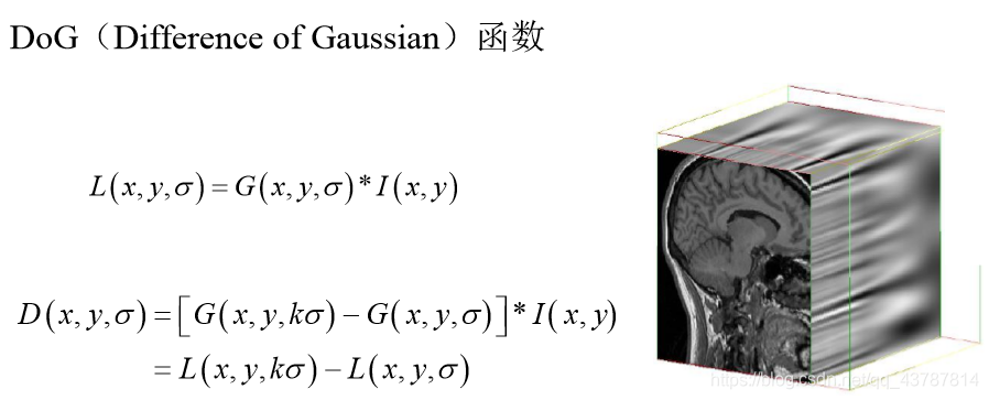
1.3.2.关键点检测-Dog
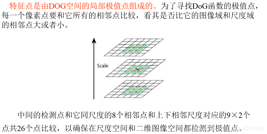
1.Dog的局部极值点
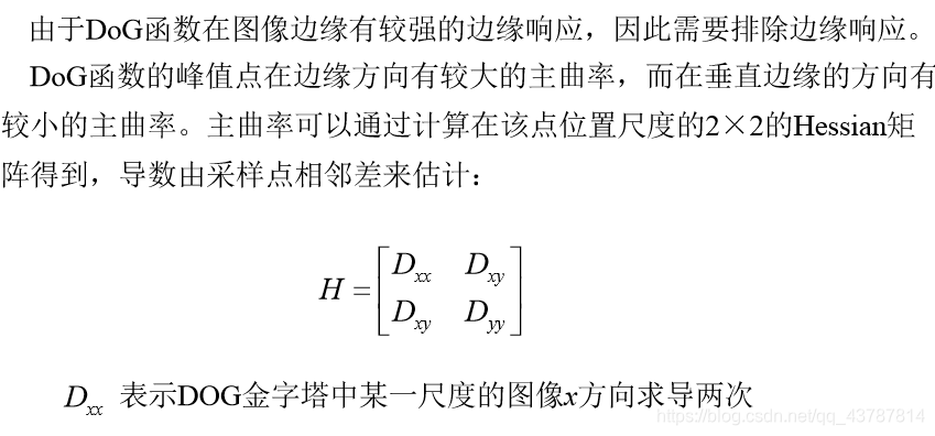
2.去除边缘响应
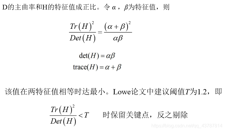
2.检测感兴趣点(例题)
# -*- coding: utf-8 -*-from PIL import Image
from pylab import *
from PCV.localdescriptors import sift
from PCV.localdescriptors import harris
# 添加中文字体支持
from matplotlib.font_manager import FontProperties
font = FontProperties(fname=r"c:\windows\fonts\SimSun.ttc", size=14)
imname = 'D:/xjx\pythonCode/pcv_data/data/empire.jpg'
im = array(Image.open(imname).convert('L'))
sift.process_image(imname, 'empire.sift')
l1, d1 = sift.read_features_from_file('empire.sift')
figure()
gray()
subplot(131)
sift.plot_features(im, l1, circle=False)
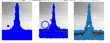
title(u'SIFT特征',fontproperties=font)
subplot(132)
sift.plot_features(im, l1, circle=True)
title(u'用圆圈表示SIFT特征尺度',fontproperties=font)
# 检测harris角点
harrisim = harris.compute_harris_response(im)
subplot(133)
filtered_coords = harris.get_harris_points(harrisim, 6, 0.1)
imshow(im)
plot([p[1] for p in filtered_coords], [p[0] for p in filtered_coords], '*')
axis('off')
title(u'Harris角点',fontproperties=font)
show()
3.描述子匹配(例题)
# -*- coding: utf-8 -*-
from PIL import Image
from pylab import *
import sys
from PCV.localdescriptors import sift
if len(sys.argv) >= 3:
im1f, im2f = sys.argv[1], sys.argv[2]
else:
# im1f = '../data/sf_view1.jpg'
# im2f = '../data/sf_view2.jpg'
im1f = 'D:/xjx\pythonCode/pcv_data/data/crans_1_small.jpg'
im2f = 'D:/xjx\pythonCode/pcv_data/data/crans_2_small.jpg'
# im1f = '../data/climbing_1_small.jpg'
# im2f = '../data/climbing_2_small.jpg'
im1 = array(Image.open(im1f))
im2 = array(Image.open(im2f))
sift.process_image(im1f, 'out_sift_1.txt')
l1, d1 = sift.read_features_from_file('out_sift_1.txt')
figure()
gray()
subplot(121)
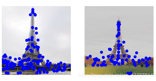
sift.plot_features(im1, l1, circle=False)
sift.process_image(im2f, 'out_sift_2.txt')
l2, d2 = sift.read_features_from_file('out_sift_2.txt')
subplot(122)
sift.plot_features(im2, l2, circle=False)
#matches = sift.match(d1, d2)
matches = sift.match_twosided(d1, d2)
print '{} matches'.format(len(matches.nonzero()[0]))
figure()
gray()
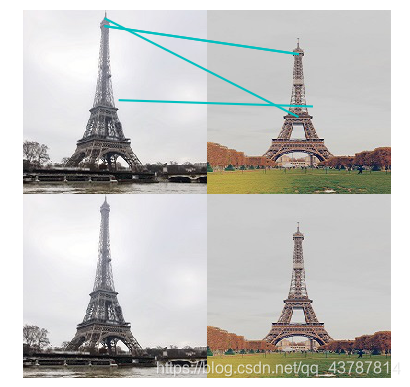
sift.plot_matches(im1, im2, l1, l2, matches, show_below=True)
show()
二.SIFT特征提取与检索(实验)
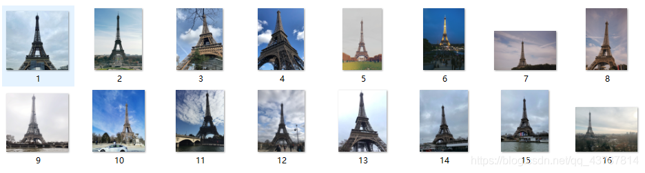
1. 数据集准备
2. 特征提取
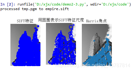
2.1 运行结果
2.2 分析
由实验结果可知,SIFT算法具有较好的稳定性和不变性,能够适应旋转、尺度缩放、亮度的变化,能在一定程度上不受视角变化、仿射变换、噪声的干扰。还具有多量性,就算只有单个物体,也能产生大量特征向量
对比SIFT特征提取与Harris角点检测结果,可以看出Harris角点检测算法提取出的特征点明显低于SIFT算法。对于比较平坦的区域,Harris角点检测算法能检测到的特征点很少甚至没有。故而,由于无法检测到足够的特征点,Harris角点检测算法在特征点有效性、计算时效性以及特征点相似不变性三个方面均不如SIFT算法显的高效。
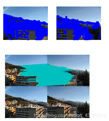
3. 描述子匹配
4. 输出匹配图片
4. 1 代码
from PIL import Image
from pylab import *
from PCV.localdescriptors import sift
import matplotlib.pyplot as plt


im1f = 'D:/python/images/test_3/11.jpg'
im1 = array(Image.open(im1f))
sift.process_image(im1f, 'out_sift_1.txt')
l1, d1 = sift.read_features_from_file('out_sift_1.txt')

arr=[]
arrHash = {}
for i in range(1,15):

    im2f = (r'D:/python/images/test_3/'+str(i)+'.jpg')
    im2 = array(Image.open(im2f))
    sift.process_image(im2f, 'out_sift_2.txt')
    l2, d2 = sift.read_features_from_file('out_sift_2.txt')
    matches = sift.match_twosided(d1, d2)
    length=len(matches.nonzero()[0])
    length=int(length)
    arr.append(length)
    arrHash[length]=im2f

arr.sort()
arr=arr[::-1]
arr=arr[:3]
i=0
plt.figure(figsize=(5,12))
for item in arr:
    if(arrHash.get(item)!=None):
        img=arrHash.get(item)
        im1 = array(Image.open(img))
        ax=plt.subplot(511 + i)
        ax.set_title('{} matches'.format(item))
        plt.axis('off')
        imshow(im1)
        i = i + 1

plt.show()
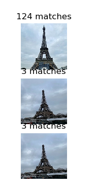
4. 2 运行结果
输入:
输出:
三. 地理标记图像匹配
3.1 代码
# -*- coding: utf-8 -*-
from pylab import *
from PIL import Image
from PCV.localdescriptors import sift
from PCV.tools import imtools
import pydot

""" This is the example graph illustration of matching images from Figure 2-10.
To download the images, see ch2_download_panoramio.py."""

#download_path = "panoimages"  # set this to the path where you downloaded the panoramio images
#path = "/FULLPATH/panoimages/"  # path to save thumbnails (pydot needs the full system path)

download_path = "F:/dropbox/Dropbox/translation/pcv-notebook/data/panoimages"  # set this to the path where you downloaded the panoramio images
path = "F:/dropbox/Dropbox/translation/pcv-notebook/data/panoimages/"  # path to save thumbnails (pydot needs the full system path)

# list of downloaded filenames
imlist = imtools.get_imlist(download_path)
nbr_images = len(imlist)

# extract features
featlist = [imname[:-3] + 'sift' for imname in imlist]
for i, imname in enumerate(imlist):
    sift.process_image(imname, featlist[i])

matchscores = zeros((nbr_images, nbr_images))

for i in range(nbr_images):
    for j in range(i, nbr_images):  # only compute upper triangle
        print 'comparing ', imlist[i], imlist[j]
        l1, d1 = sift.read_features_from_file(featlist[i])
        l2, d2 = sift.read_features_from_file(featlist[j])
        matches = sift.match_twosided(d1, d2)
        nbr_matches = sum(matches > 0)
        print 'number of matches = ', nbr_matches
        matchscores[i, j] = nbr_matches
print "The match scores is: \n", matchscores

# copy values
for i in range(nbr_images):
    for j in range(i + 1, nbr_images):  # no need to copy diagonal
        matchscores[j, i] = matchscores[i, j]

#可视化

threshold = 2  # min number of matches needed to create link

g = pydot.Dot(graph_type='graph')  # don't want the default directed graph

for i in range(nbr_images):
    for j in range(i + 1, nbr_images):
        if matchscores[i, j] > threshold:
            # first image in pair
            im = Image.open(imlist[i])
            im.thumbnail((100, 100))
            filename = path + str(i) + '.png'
            im.save(filename)  # need temporary files of the right size
            g.add_node(pydot.Node(str(i), fontcolor='transparent', shape='rectangle', image=filename))

            # second image in pair
            im = Image.open(imlist[j])
            im.thumbnail((100, 100))
            filename = path + str(j) + '.png'
            im.save(filename)  # need temporary files of the right size
            g.add_node(pydot.Node(str(j), fontcolor='transparent', shape='rectangle', image=filename))

            g.add_edge(pydot.Edge(str(i), str(j)))
g.write_png('whitehouse.png')
3.2 运行结果
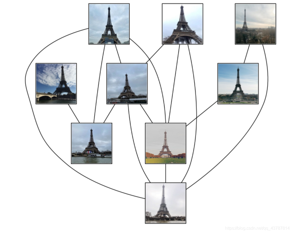
- 观察结果可知,数据集中只有9张图片形成关联,其他图片未形成关联,问题大概是所选图片数据集的不太好,导致结果误差偏大。
- 图片光线明暗和遮挡物以及角度对结果也颇有影响,较暗图片几乎都没有关联匹配的图片。
四. 实验中遇到的问题和得出的结论
问题
- 因为家里实在没有适合的场景可供拍摄,所以网上搜索的图匹配效果不那么好,影响了实验效果
- 图片开始像素过多, 导致程序运行电脑多次卡机,修改像素后有所改善
- 某些图片像素值不一样 ,导致图片无法匹配
- 安装pydot中出现诸多问题,应该先安装graphviz软件,再安装Pydot
(安装详细过程可参考详细教程)
结论
- SIFT特征不只具有尺度不变性,即使改变旋转角度,图像亮度或拍摄视角,仍然能够得到好的检测效果。
- SIFT独特性好,信息量丰富,适合于在海量特征数据库中进行快速、准确的匹配。
- SIFT有多量性,即使少数的几个物体也可以产生大量的SIFT特征向量。
- 相比于Harris角点检测,SIFT特征提取在特征点有效性、计算时效性以及特征点相似不变性几个方面都较为高效。
五. RANSAC原理及运用
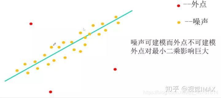
5.1 RANSAC——随机一致性采样
RANSAC主要解决样本中的外点问题,最多可处理50%的外点情况。
(1) 基本思想
RANSAC通过反复选择数据中的一组随机子集来达成目标。被选取的子集被假设为局内点,并用下述方法进行验证:
- 有一个模型适用于假设的局内点,即所有的未知参数都能从假设的局内点计算得出。
- 用1中得到的模型去测试所有的其它数据,如果某个点适用于估计的模型,认为它也是局内点。
- 如果有足够多的点被归类为假设的局内点,那么估计的模型就足够合理。
- 然后,用所有假设的局内点去重新估计模型,因为它仅仅被初始的假设局内点估计过。
- 最后,通过估计局内点与模型的错误率来评估模型。
这个过程被重复执行固定的次数,每次产生的模型要么因为局内点太少而被舍弃,要么因为它比现有的模型更好而被选用。
(2) 步骤
- 随机选择四对匹配特征
- 根据DLT计算单应矩阵 H (唯一解)
- 对所有匹配点,计算映射误差ε= ||pi’, H pi||
- 根据误差阈值,确定inliers(例如3-5像素)
- 针对最大inliers集合,重新计算单应矩阵 H
5.2 示例
1.在给定若干二维空间中的点,求直线 y=ax+b ,使得该直线对空间点的拟合误差最小。
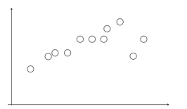
2.随机选择两个点,根据这两个点构造直线,再计算剩余点到该直线的距离
给定阈值(距离小于设置的阈值的点为inliers),计算inliers数量
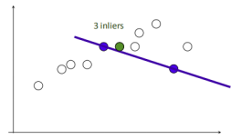
3.再随机选取两个点,同样计算inliers数量
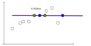
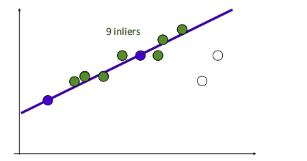
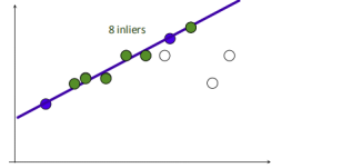
4.循环迭代,其中inliers最大的点集即为最大一致集,最后将该最大一致集里面的点利用最小二乘拟合出一条直线。
5.3 使用RANSAC算法匹配
5.3.1 源代码
# ch3_panorama_test.py
from pylab import *
from numpy import *
from PIL import Image

# If you have PCV installed, these imports should work
from PCV.geometry import homography, warp
from PCV.localdescriptors import sift

import os
root=os.getcwd()+"\\"

"""
This is the panorama example from section 3.3.
"""

# set paths to data folder
featname = ['../data/wanren/uu' + str(i + 1) + '.sift' for i in range(5)]
imname = ['../data/wanren/uu' + str(i + 1) + '.jpg' for i in range(5)]

# extract features and match
l = {}
d = {}
for i in range(5):
    sift.process_image(root+imname[i], root+featname[i])
    l[i], d[i] = sift.read_features_from_file(featname[i])

matches = {}
for i in range(4):
    matches[i] = sift.match(d[i + 1], d[i])

# visualize the matches (Figure 3-11 in the book)
for i in range(4):
    im1 = array(Image.open(imname[i]))
    im2 = array(Image.open(imname[i + 1]))
    figure()
    sift.plot_matches(im2, im1, l[i + 1], l[i], matches[i], show_below=True)


# function to convert the matches to hom. points
def convert_points(j):
    ndx = matches[j].nonzero()[0]
    fp = homography.make_homog(l[j + 1][ndx, :2].T)
    ndx2 = [int(matches[j][i]) for i in ndx]
    tp = homography.make_homog(l[j][ndx2, :2].T)

    # switch x and y - TODO this should move elsewhere
    fp = vstack([fp[1], fp[0], fp[2]])
    tp = vstack([tp[1], tp[0], tp[2]])
    return fp, tp


# estimate the homographies
model = homography.RansacModel()

fp, tp = convert_points(1)
H_12 = homography.H_from_ransac(fp, tp, model)[0]  # im 1 to 2

fp, tp = convert_points(0)
H_01 = homography.H_from_ransac(fp, tp, model)[0]  # im 0 to 1

tp, fp = convert_points(2)  # NB: reverse order
H_32 = homography.H_from_ransac(fp, tp, model)[0]  # im 3 to 2

tp, fp = convert_points(3)  # NB: reverse order
H_43 = homography.H_from_ransac(fp, tp, model)[0]  # im 4 to 3

# warp the images
delta = 2000  # for padding and translation

im1 = array(Image.open(imname[1]), "uint8")
im2 = array(Image.open(imname[2]), "uint8")
im_12 = warp.panorama(H_12, im1, im2, delta, delta)

im1 = array(Image.open(imname[0]), "f")
im_02 = warp.panorama(dot(H_12, H_01), im1, im_12, delta, delta)

im1 = array(Image.open(imname[3]), "f")
im_32 = warp.panorama(H_32, im1, im_02, delta, delta)

im1 = array(Image.open(imname[4]), "f")
im_42 = warp.panorama(dot(H_32, H_43), im1, im_32, delta, 2 * delta)

figure()
imshow(array(im_42, "uint8"))
axis('off')
savefig("quanjing.png", dpi=300)
show()
5.3.2 结果分析
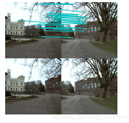
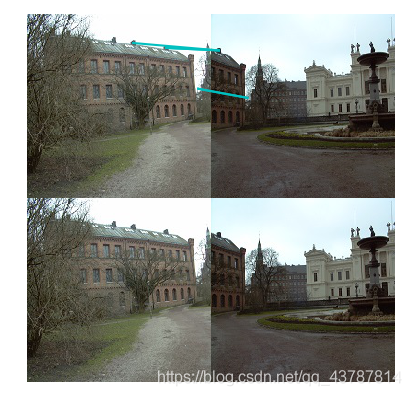
景深丰富:
有RANSAC:
第一组:
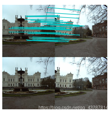
第二组:
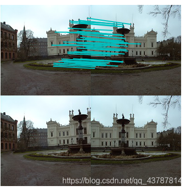
第三组:
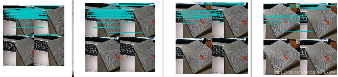
无RANSAC的第一组匹配结果:
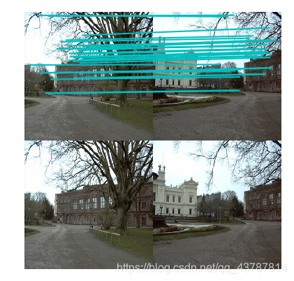
此结果显示特征匹配不够细致
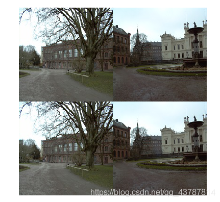
景深单一:
有RANSAC:
景深单一匹配到的特征较少,且此组照片不能拼接,暂且不知原因;
无RANSAC:
结果显示0匹配;
实验遇到的问题:
多组实验图片拼接效果都不理想,黑暗区域较多,原因暂且未知,或许是拍摄手法的问题。
实验拼接效果的数据集: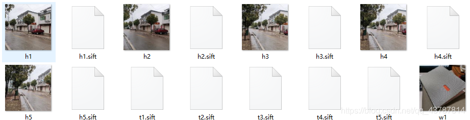
结果:
???
经多次试验结果归纳及对比可知:
- 在运用RANSAC 的算法中,景深丰富的场景匹配效果更精确,错误匹配减少;
- 未运用RANSAC的算法中,景深单一的场景甚至匹配不到特征,但运用RANSAC后,可精确匹配少数特征,但差别不大;
- 可知RANSAC不仅能删除错误匹配,在细节处理方面也更细致;