数据科学与机器学习案例之WiFi定位系统的位置预测
数据简介
可供建模的训练集与测试集共有140多万条记录,我们对文本数据进行了转换,开发了文本处理的函数,并进行了程序调试。
汇总之后的数据共有以下字段:时间、WiFi地址、X、Y、方向、移动设备地址、信号值、信号频率、距离
| 数据变量 | 类型 |
|---|---|
时间 | POSIXct |
WiFi地址 | 分类 |
X | 连续 |
Y | 连续 |
Z | 连续 |
方向 | 连续 |
移动设备地址 | 分类 |
信号值 | 连续 |
信号频率 | 分类 |
距离 | 连续 |
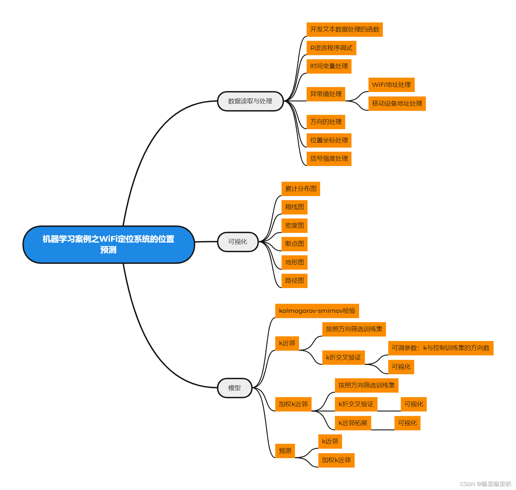
详细的数据处理、数据汇总、可视化、模型、预测已在思维导图中说明。以下就不在单独详细介绍。
可视化图集

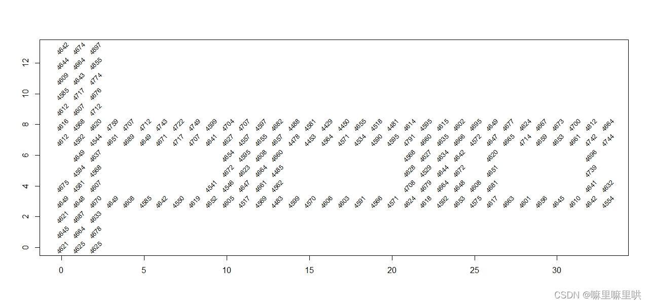
不同位置的记录数
可视化图集1
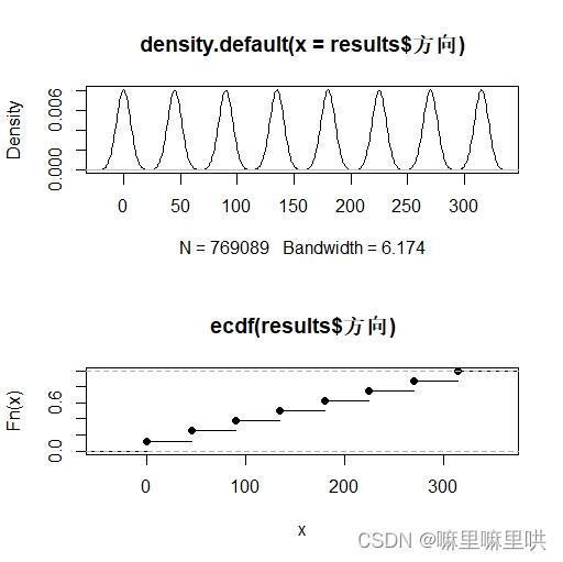 图1 训练数据的方向的密度图与累积分布图 图1 训练数据的方向的密度图与累积分布图
|
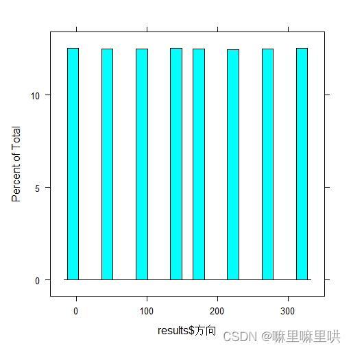 图2 训练数据方向的直方图 图2 训练数据方向的直方图
|
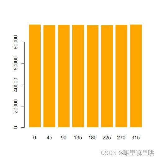 图3 训练数据方向的柱状图 图3 训练数据方向的柱状图
|
 图4 不同数据分割情形下数目与均值减中位数的散点图与拟合估计图 图4 不同数据分割情形下数目与均值减中位数的散点图与拟合估计图
|
可视化图集2
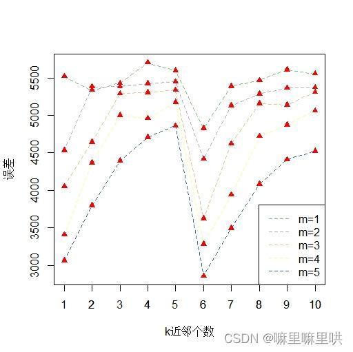 图1 k近邻交叉验证图 图1 k近邻交叉验证图
|
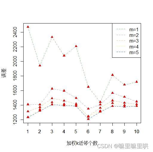 图2 加权k近邻交叉验证图 图2 加权k近邻交叉验证图
|
 图3 直接预测的原始位置与预测位置的路径图 图3 直接预测的原始位置与预测位置的路径图
|
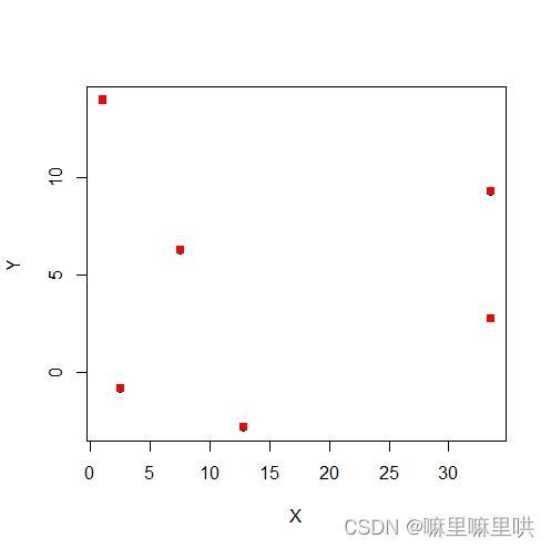 图4 WiFi位置图 图4 WiFi位置图
|
可视化图集3
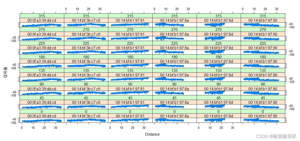
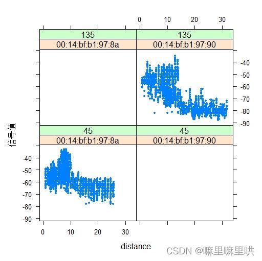 图1 训练数据中特定筛选条件下的散点图 图1 训练数据中特定筛选条件下的散点图
|
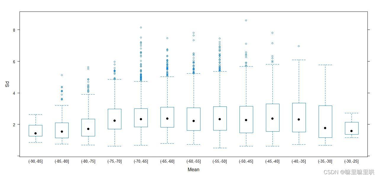
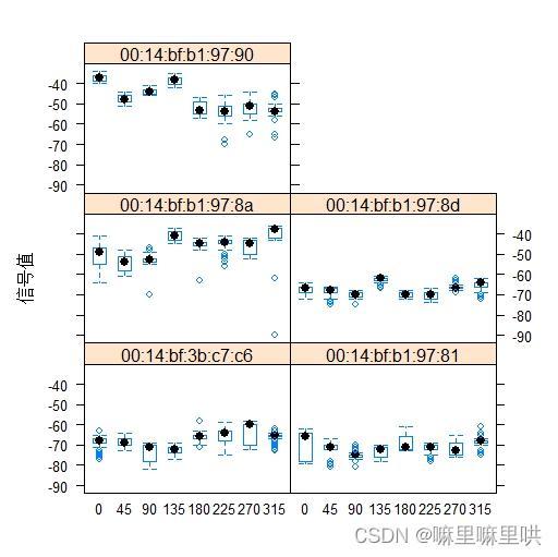 图2 特定筛选条件下的信号值的箱线图 图2 特定筛选条件下的信号值的箱线图
|
可视化图集4
代码汇总
> library(ggplot2)
> library(caret)
> library(data.table)
> library(parallel)
> library(lubridate)
>
> txt = readLines('训练.txt')
>
> head(txt,6)
>
> process.data <- function(x){
+ a = strsplit(x,'[,;=]')[[1]]
+ mat = matrix(a[-(1:10)],ncol = 4,byrow = T)
+ result = cbind(matrix(a[c(2,4,6,7,8,10)],nrow = nrow(mat),ncol = 6
+ ,byrow = T),mat)
+ result}
>
> process.data(txt[14])
>
> a1 = lapply(txt[4:20],process.data)
>
> results = lapply(txt[substr(txt,1,1) != '#'],process.data)
>
> options(error = recover,warn = 2)
>
> process.data <- function(x){
+ a = strsplit(x,'[,;=]')[[1]]
+ if(length(a) == 10) return(NULL)
+ mat = matrix(a[-(1:10)],ncol = 4,byrow = T)
+ result = cbind(matrix(a[c(2,4,6,7,8,10)],nrow = nrow(mat),
+ ncol = 6,byrow = T),mat)
+ result}
>
> results = lapply(txt[substr(txt,1,1) != '#'],process.data)
>
> options(error = recover,warn = 1)
>
> results = as.data.frame(do.call('rbind',results),stringsAsFactors = FALSE)
>
> colnames(results) = c('时间','WiFi地址','X','Y','Z','方向',
+ '移动设备地址','信号值','信号频率','模式')
>
> results[c('时间','X','Y','Z','方向','信号值')] = lapply(results[c('时间','X','Y','Z','方向','信号值')],as.numeric)
>
# 删除类型变量
>
> results = results[results$模式 == '3',]
> results = results[,'模式' != names(results)]
>
> results$时间 = results$时间 / 1000
> class(results$时间) = c('POSIXT','POSIXct')
>
> start = c(seq(1,length(results$时间),by = 10000))
> end = c(start[2:length(start)]-1,length(results$时间))
>
> for(i in 1:length(start)){
+ sink('Time.txt',append = T)
+ print(results$时间[start[i]:end[i]])
+ sink() }
>
> Time = readLines('Time.txt')
> strsplit(Time[1],'[\\"]')[[1]][c(2,4)]
>
> BI = function(x){
+ a = strsplit(x,'[\\"]')[[1]][c(2,4)]
+ a = gsub(' CST','',a)
+ a}
> time = unlist(lapply(Time,BI))
> time = time[-length(time)]
>
> results$时间 = time
>
> results$时间 = as.POSIXct(results$时间)
> results$时间 <- update(results$时间, year=2021)
>
> summary(results[,c('时间','X','Y','Z','方向','信号值')])
>
>
> table(results$WiFi地址)
>
> sort(table(results$移动设备地址),T)[1:6]
> names(sort(table(results$移动设备地址),T)[1:6])
>
> histogram(results$方向)
>
> opar = par(mfrow = c(2,1))
> plot(density(results$方向))
> plot(ecdf(results$方向))
> par(opar)
>
> angle.res <- function(x){
+ angles = seq(0,by = 45,length = 9)
+ a = sapply(x,function(y){
+ which.min(abs(y - angles))})
+ c(angles[1:8],0)[a]
+ }
>
> results$方向 = angle.res(results$方向)
>
> barplot(table(results$方向),names.arg = names(table(results$方向)),
+ col = 'orange', # 填充颜色
+ border = '#ffffff')
>
> c(length(unique(results$移动设备地址)),length(unique(results$信号频率)))
>
> t = sort(table(results$移动设备地址),T)
>
> results = results[which(results$移动设备地址 %in% names(t)[1:8]),]
>
# 检查移动设备地址与频率之间是否是一一对应关系
>
> data = with(results,table(移动设备地址,信号频率))
>
> apply(data,2,function(x) sum(x > 0))
>
> temp = temp[temp$移动设备地址 == '00:0f:a3:39:e0:4b' & temp$信号频率 == '2462000000',]
>
> results = results[results$移动设备地址 != '00:0f:a3:39:e0:4b' & results$信号频率 != '2462000000',]
>
> location = with(results,by(results,list(X,Y),function(x) x))
>
> (sapply(location,class))
> sum(sapply(location,class) == 'NULL')
> location = location[! (sapply(location,class) == 'NULL')]
> length(location)
>
> sapply(location,class)
> sapply(location,nrow) # 每个坐标下的记录
>
>
> lp = sapply(location,function(x) c(unique(x$X),unique(x$Y)))
> lp <- rbind(lp,sapply(location,nrow))
>
> plot(t(lp),type = 'n',xlab = '',ylab = '')
> text(t(lp),labels = t(lp)[,3],cex = .8,srt = 45)
>
> lattice::bwplot(信号值 ~ factor(方向) | 移动设备地址,data = results,
+ subset = X == 2 & Y == 12 & 移动设备地址 != '00:0f:a3:39:dd:cd',
+ layout = c(2,3)) # 信号强度的分布
>
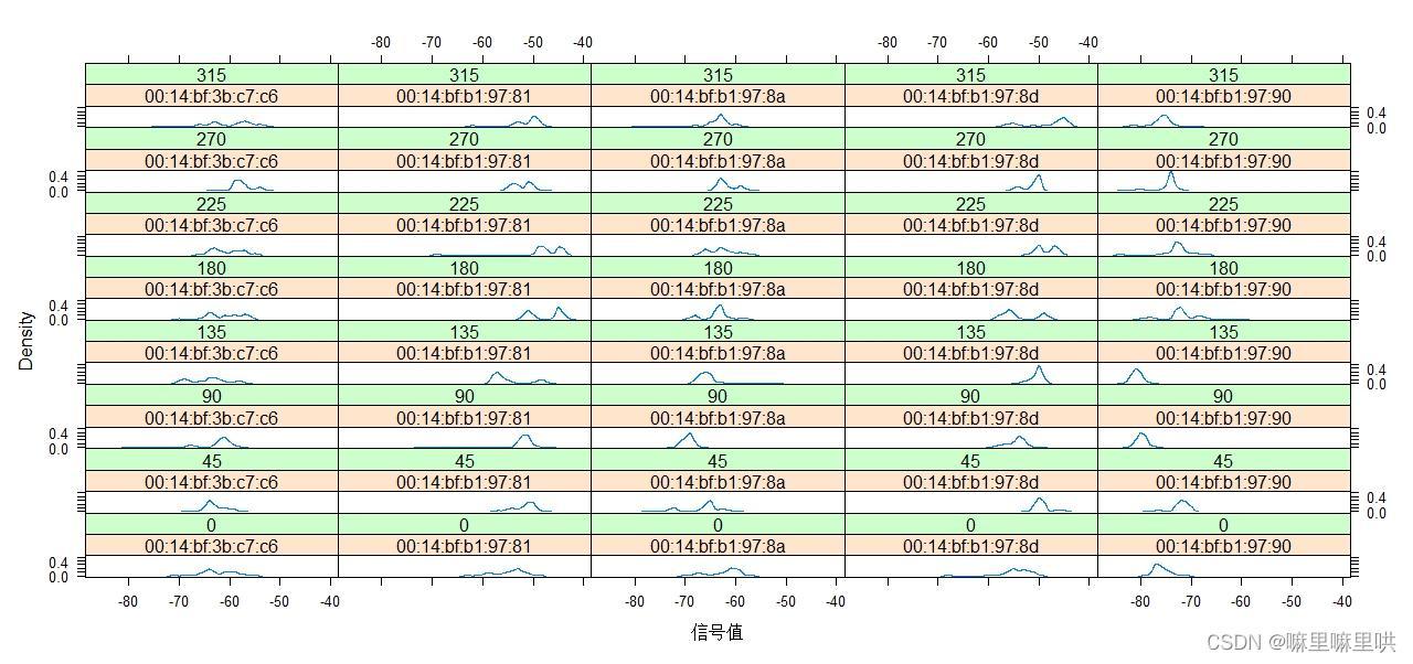
> lattice::densityplot(~信号值 | 移动设备地址 + factor(方向),data = results,
+ subset = X == 24 & Y == 4 &
+ 移动设备地址 != "00:0f:a3:39:dd:cd",
+ bw = 0.5, plot.points = FALSE)
>
> results$XY = paste(results$X,results$Y,sep = '-')
>
> XYanglelocation = with(results,by(results,list(XY,方向,移动设备地址),function(x)x))
>
>
> temp1 = lapply(XYanglelocation,function(x){
+ and = x[1,]
+ and$Mean = mean(x$信号值)
+ and$Median = median(x$信号值)
+ and$IQR = IQR(x$信号值)
+ and$num = length(x$信号值)
+ and$sd = sd(x$信号值)
+ and}) # 汇总
> temp1 = do.call('rbind',temp1)
>
>
> breaks = seq(-90,-25,by = 5)
> lattice::bwplot(sd ~ cut(Mean,breaks = breaks),data = temp1,
+ xlab = 'Mean',ylab = 'Sd')
>
> with(temp1,smoothScatter((Mean - Median) ~ num,
+ xlab = 'Num',ylab = 'Mean - Median'))
> abline(h = 0,col = '#984ea3',lwd = 2)
>
> loess.and = with(temp1,loess(diff ~ num ,data = data.frame(diff = Mean - Median,
+ num = num)))
>
> loess.pre = predict(loess.and,newdata = data.frame(num = 60:120))
>
> with(temp1,smoothScatter((Mean - Median) ~ num,
+ xlab = 'Num',ylab = 'Mean - Median'))
> abline(h = 0,col = '#984ea3',lwd = 2)
> lines(x = 60:120,y = loess.pre)
> points(x = 60:120,y = loess.pre)
>
> onelocationangle = subset(temp1,
+ 移动设备地址 == '00:14:bf:b1:97:8d' & 方向 == 0)
>
> smooth1 = fields::Tps(onelocationangle[,c('X','Y')],onelocationangle$Mean)
>
> smooth1 = fields::predictSurface(smooth1)
> fields::plot.surface(smooth1,type = 'C')
> points(x = onelocationangle[,'X'],y = onelocationangle[,'Y'],
+ pch = 19,cex = .5) # 地形图
>
# 构造函数
>
> surface = function(data,location,angle = 45){
+ library(fields)
+ onelocationangle = subset(data,
+ data$移动设备地址 == location & data$方向 == angle)
+ smooth1 = Tps(onelocationangle[,c('X','Y')],onelocationangle$Mean)
+ smooth1 = predictSurface(smooth1)
+ plot.surface(smooth1,type = 'C')
+ points(x = onelocationangle[,'X'],y = onelocationangle[,'Y'],
+ pch = 19,cex = .5) }
>
> surface(temp1,'00:14:bf:b1:97:90')
>
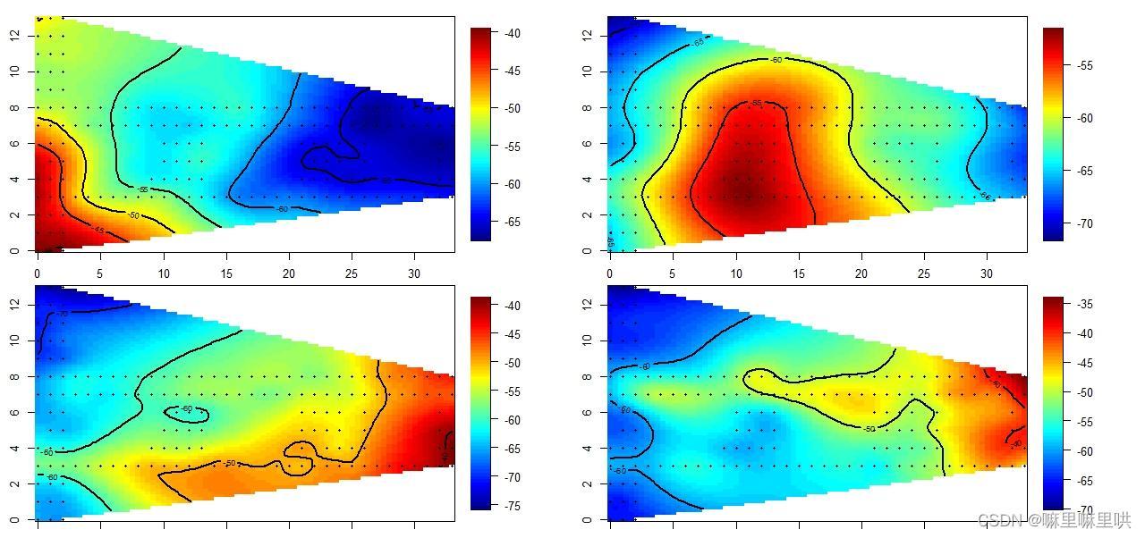
> opar = par(mfrow = c(2,2),mar = rep(1,4))
> mapply(surface,data = list(temp1),
+ location = sample(unique(temp1$移动设备地址),4),
+ angle = rep(c(45,135),each = 2)) # 地形图
> par(opar)
>
> WiFi.matrix = matrix(c( 7.5, 6.3, 2.5, -.8, 12.8, -2.8,
+ 1, 14, 33.5, 9.3, 33.5, 2.8),
+ ncol = 2,byrow = T,
+ dimnames = list(unique(results$移动设备地址),c('x','y')))
>
> diffs = results[,c('X','Y')] - WiFi.matrix[results$移动设备地址,]
>
> results$distance = sqrt(diffs[,1] ^2 + diffs[,2]^2)
>
> lattice::xyplot(信号值 ~ distance | factor(移动设备地址) + factor(方向),
+ data = results,pch = 19,cex = .5,xlab = 'Distance')
>
> lattice::xyplot(信号值 ~ distance | factor(移动设备地址) + factor(方向),
+ data = results,
+ subset = 移动设备地址 == c("00:14:bf:b1:97:8a","00:14:bf:b1:97:90")&
+ 方向 == c(45,135),pch = 19,cex = .5)
>
> txt1 = readLines('测试.txt')
>
> options(error = recover,warn = 2)
> process.data = function(x){
+ a = strsplit(x,'[,;=]')[[1]]
+ if(length(a) <= 10) return(NULL)
+ mat = matrix(a[-(1:10)],ncol = 4,byrow = T)
+ result = cbind(matrix(a[c(2,4,6,7,8,10)],nrow = nrow(mat),
+ ncol = 6,byrow = T),mat)
+ result}
> test = lapply(txt1,process.data)
> test = as.data.frame(do.call('rbind',test))
>
>
> colnames(test) = c('时间','WiFi地址','X','Y','Z','方向',
+ '移动设备地址','信号值','信号频率','模式')
>
> test[c('时间','X','Y','Z','方向','信号值')] = lapply(test[c('时间','X','Y','Z','方向','信号值')],as.numeric)
>
# 删除类型变量
>
> test = test[test$模式 == '3',]
> test = test[,'模式' != names(test)]
>
> test$时间 = test$时间 / 1000
> class(test$时间) = c('POSIXT','POSIXct')
>
> start = c(seq(1,length(test$时间),by = 10000))
> end = c(start[2:length(start)]-1,length(test$时间))
>
> for(i in 1:length(start)){
+ sink('Time1.txt',append = T)
+ print(results$时间[start[i]:end[i]])
+ sink() }
>
> Time1 = readLines('Time1.txt')
> strsplit(Time[1],'[\\"]')[[1]][c(2,4)]
>
> BI = function(x){
+ a = strsplit(x,'[\\"]')[[1]][c(2,4)]
+ a = gsub(' CST','',a)
+ a}
> time1 = unlist(lapply(Time1,BI))
> time1 = time1[-length(time1)]
>
> test$时间 = time1
>
> test$时间 = as.POSIXct(test$时间)
> test$时间 <- update(test$时间, year=2021)
>
> summary(test[,c('时间','X','Y','Z','方向','信号值')])
>
>
> angle.res <- function(x){
+ angles = seq(0,by = 45,length = 9)
+ a = sapply(x,function(y){
+ which.min(abs(y - angles))})
+ c(angles[1:8],0)[a]
+ }
>
> test$方向 = angle.res(test$方向)
>
> class(with(test,table(移动设备地址,信号频率)))
>
> apply(with(test,table(移动设备地址,信号频率)),2,function(x) sum(x > 0))
>
# 修改
>
>
> test$移动设备地址[which(test$移动设备地址 == '00:0f:a3:39:e0:4b' &
+ test$信号频率 == '2462000000')] = '00:0f:a3:39:e1:c0'
> test$移动设备地址[which(test$移动设备地址 == '00:0f:a3:39:e2:10' &
+ test$信号频率 == '2437000000')] = '00:14:bf:b1:97:8a'
>
> test = test[which(test$移动设备地址 %in% unique(results$移动设备地址)),]
>
> test$XY = paste(test$X,test$Y,sep = '-')
>
> with(test,table(XY,方向))
>
> variables = c('X','Y','方向','XY')
> test.XY = with(test,by(test,list(XY),function(x) {
+ as = x[1,variables]
+ Mean = tapply(x$信号值,x$移动设备地址,mean)
+ x = matrix(Mean,nrow = 1,ncol = 6,dimnames = list(
+ as$XY,names(Mean)))
+ cbind(as,x) }))
> test.XY = do.call('rbind',test.XY)
>
# 根据角度以及m选择训练数据集的数据
>
> names(test.XY)
> m = 3
> angleNewobs = 230
> rfs = seq(0,by = 45,length = 8)
> nearangle = angle.res(angleNewobs)
>
> if(m %% 2 == 1){# 选择奇数个近邻
+ angles = seq(-45 * (m-1) / 2,45 * (m-1) / 2,length = m)
+ } else { # 选择偶数个近邻
+ m = m+1
+ angles = seq(-45 * (m-1) / 2,45 * (m-1) / 2,length = m)
+ if(sign(angleNewobs-nearangle) > -1){
+ angles = angles[-1]}
+ else {
+ angles = angles[-m]}
+ }
> angles = angles + nearangle
> angles[angles < 0] = angles[angles < 0] + 360
> angles[angles > 360] = angles[angles > 360] - 360
>
>
> resize = function(data,var = 'Mean',keep = c('X','Y','XY')){
+ ans = with(data,by(data,list(XY),function(x){
+ as = x[1,keep]
+ y = tapply(x[,var],x$移动设备地址,mean)
+ A = matrix(y,nrow = 1,ncol = 6,
+ dimnames = list(as$XY,
+ names(y)))
+ cbind(as,A)}))
+ newdata = do.call('rbind',ans)
+ return(newdata)}
>
# 根据角度选择训练集
>
> select.train = function(angleNewobs,data,m = 1){
+ rfs = seq(0,by = 45,length = 8)
+ nearangle = angle.res(angleNewobs)
+
+ if(m %% 2 == 1){# 选择奇数个近邻
+ angles = seq(-45 * (m-1) / 2,45 * (m-1) / 2,length = m)
+ } else { # 选择偶数个近邻
+ m = m+1
+ angles = seq(-45 * (m-1) / 2,45 * (m-1) / 2,length = m)
+ if(sign(angleNewobs-nearangle) > -1){
+ angles = angles[-1]}
+ else {
+ angles = angles[-m]}
+ }
+ angles = angles + nearangle
+ angles[angles < 0] = angles[angles < 0] + 360
+ angles[angles > 360] = angles[angles > 360] - 360
+
+ angles = sort(angles)
+ train.subset = data[data$方向 %in% angles,]
+ resize(train.subset) }
>
> train.1 = select.train(130,temp1,m=1)
> train.2 = select.train(130,temp1,m=2)
>
> findnn = function(newsignal,train.subset){
+ diffs = apply(train.subset[,5:10],1,function(x)
+ x - newsignal)
+ distance = apply(diffs,2,function(x) sqrt(sum(x)^2))
+ closest = order(distance)
+ return(train.subset[closest,1:3]) } # 按照距离的长短排列(k近邻)
>
> pred.XY = function(newSignals, newAngles, trainData,
+ numAngles = 1, k = 3){
+
+ closeXY = list(length = nrow(newSignals))
+
+ for (i in 1:nrow(newSignals)) {
+ trainSS = select.train(newAngles[i], trainData, m = numAngles) # 筛选不同的训练集
+ closeXY[[i]] =
+ findnn(newsignal = as.numeric(newSignals[i, ]), trainSS) # 储存数据框
+ }
+ estXY = lapply(closeXY,
+ function(x) sapply(x[ , 1:2],
+ function(x) mean(x[1:k]))) # 按照第k个近邻计算
+ estXY = do.call("rbind", estXY)
+ return(estXY)
+ }
>
> final1.1 = pred.XY(test.XY[,5:10],test.XY[,3],temp1) # 角度数1,3近邻
>
> plot(x = test.XY[,1],y = test.XY[,2],type = 'n',xlim = range(test.XY[,1]),
+ ylim = range(test.XY[,2]),xlab = 'X',ylab = 'Y')
> points(x = test.XY[,1],y = test.XY[,2],col = 'black',pch = 16)
> points(x = final1.1[,1],y = final1.1[,2],col = 'red',pch = 16)
>
>
> A = vector(mode = 'list',length = 25)
> df = vector(mode = 'numeric',length = 25)
> error.cal = function(Matrix){
+ res = sum(rowSums((Matrix - test.XY[,c('X','Y')])^2))
+ res}
>
> knn.grid = expand.grid(m = 1:5,k = 1:5)
>
> for(i in 1:length(A)){
+ A[[i]] = pred.XY(test.XY[,5:10],test.XY[,3],temp1,knn.grid[i,1],
+ knn.grid[i,2])
+ df[i] = error.cal(A[[i]]) }
>
> a1 = pred.XY(test.XY[,5:10],test.XY[,3],temp1,knn.grid[1,1],knn.grid[1,2])
>
> barplot(df)
> knn.grid[which.min(df),]
>
# 可视化
>
> plot(x = test.XY[,'X'],y = test.XY[,'Y'],xlim = range(test.XY[,'X']),
+ ylim = range(test.XY[,'Y']),xlab = 'X',ylab = 'Y',type = 'n')
> box()
> points(x = test.XY[,'X'],y = test.XY[,'Y'],pch = 16,col = 'black')
> points(x = A[[14]][,1],y = A[[14]][,2],pch = 17,col = 'red')
> segments(x0 = test.XY[,'X'],y0 = test.XY[,'Y'],
+ x1 = A[[14]][,1],y1 = A[[14]][,2],lwd = 1,lty = 2,
+ col = 'grey')
> legend('topright',c('原始位置','最优预测位置m=4 k=3'),
+ pch = c(16,17),col = c('black','red'))
>
# CV交叉验证
>
> resize = function(data,keep = c('X','Y','XY','方向'),
+ angles = seq(0,by = 45,length = 8),
+ sampleangle = FALSE){
+
+ res = with(data,by(data,list(XY),function(x){
+ if(sampleangle){
+ x = x[x$方向 == sample(angles,1),]}
+ as = x[1,keep]
+ y = tapply(x$信号值,x$移动设备地址,mean)
+ A = matrix(y,nrow = 1,ncol = length(y),
+ dimnames = list(as$XY,names(y)))
+ cbind(as,A) } ))
+ newdata = do.call('rbind',res)
+ return(newdata) }
>
> v = 10
> sample.location = sample(unique(temp1$XY))
> sample.location = matrix(sample.location,ncol = v,
+ nrow = floor(length(sample.location) / v))
>
> test.cv = resize(results,sampleangle = TRUE)
>
> knn.grid = expand.grid(m = 1:5,k = 1:10)
> B = matrix(NA,nrow = nrow(knn.grid),ncol = 10)
> error.cal = function(Matrix,data){
+ res = sum(rowSums((Matrix - data)^2))
+ res}
>
> for(i in 1:v){
+ test.fold = subset(test.cv,XY %in% sample.location[,i])
+ train.fold = subset(temp1,XY %in% sample.location[,-i])
+ actual.fold = test.fold[,c('X','Y')]
+ for(j in 1:nrow(B)){
+ temp = pred.XY(test.fold[,5:10],test.fold[,4],
+ train.fold,knn.grid[j,1],knn.grid[j,2] )
+ B[j,i] = error.cal(temp,actual.fold)}
+ }
# 可视化
> y = apply(B,1,mean)
> col <- RColorBrewer::brewer.pal(8,'Accent')
> plot(x = 1:10,y = c(1:10),type = 'n',xlim = c(1,10),
ylim = range(y),xlab = 'k近邻个数',ylab = '误差')
> box()
> axis(side = 1,at = 1:10)
> lines(x = 1:10,y = y[1:10],lty = 2,lwd = 1,col = '#7FC97F')
> lines(x = 1:10,y = y[11:20],lty = 2,lwd = 1,col = '#BEAED4')
> lines(x = 1:10,y = y[21:30],lty = 2,lwd = 1,col = '#FDC086')
> lines(x = 1:10,y = y[31:40],lty = 2,lwd = 1,col = '#FFFF99')
> lines(x = 1:10,y = y[41:50],lty = 2,lwd = 1,col = '#386CB0')
> points(x = 1:10,y = y[1:10],pch = 17,col = 'red')
> points(x = 1:10,y = y[11:20],pch = 17,col = 'red')
> points(x = 1:10,y = y[21:30],pch = 17,col = 'red')
> points(x = 1:10,y = y[31:40],pch = 17,col = 'red')
> points(x = 1:10,y = y[41:50],pch = 17,col = 'red')
> legend('bottomright',c('m=1','m=2','m=3','m=4','m=5'),
+ lty = rep(2,5),lwd = rep(1,5),
+ col = col[1:5])
>
> final1 = pred.XY(newSignals = test.XY[,5:10],newAngles = test.XY[,3],
+ trainData = temp1,numAngles = 1, k = 10)
>
> err1 = error.cal(final1,test.XY[,c('X','Y')])
>
# 加权k近邻
>
> findnn = function(newsignal,train.subset){
+ diffs = apply(train.subset[,5:10],1,function(x)
+ x - newsignal)
+ distance = apply(diffs,2,function(x) sqrt(sum(x)^2))
+ train.subset$distance = round(1/distance,5)
+ closest = order(distance)
+ return(train.subset[closest,c(1:3,11)]) } # 按照距离的长短排列(k近邻)
>
> trainSS = select.train(130, temp1, m = 2)
>
> pred.XY = function(newSignals, newAngles, trainData,
+ numAngles = 1, k = 3){
+
+ closeXY = list(length = nrow(newSignals))
+
+ for (i in 1:nrow(newSignals)) {
+ trainSS = select.train(newAngles[i], trainData, m = numAngles) # 筛选不同的训练集
+ closeXY[[i]] =
+ findnn(newsignal = as.numeric(newSignals[i, ]), trainSS) # 储存数据框
+ }
+ estXY = lapply(closeXY,function(x) {
+ weights = x$distance[1:k] / sum(x$distance[1:k])
+ sapply(x[,1:2],function(x) sum(x[1:k] * weights))}) # 按照第k个近邻计算
+ estXY = do.call("rbind", estXY)
+ return(estXY)
+ }
>
> C = matrix(NA,nrow = nrow(knn.grid),ncol = 10)
> error.cal = function(Matrix,data){
+ res = sum(rowSums((Matrix - data)^2))
+ res}
>
> for(i in 1:v){
+ test.fold = subset(test.cv,XY %in% sample.location[,i])
+ train.fold = subset(temp1,XY %in% sample.location[,-i])
+ actual.fold = test.fold[,c('X','Y')]
+ for(j in 1:nrow(C)){
+ temp = pred.XY(test.fold[,5:10],test.fold[,4],
+ train.fold,knn.grid[j,1],knn.grid[j,2] )
+ C[j,i] = error.cal(temp,actual.fold)}
+ }
>
# 可视化
> y = apply(C,1,mean)
> col <- RColorBrewer::brewer.pal(8,'Accent')
> plot(x = 1:10,y = c(1:10),type = 'n',xlim = c(1,10),
+ ylim = range(y),xlab = '加权k近邻个数',ylab = '误差')
> box()
> axis(side = 1,at = 1:10)
> lines(x = 1:10,y = y[1:10],lty = 2,lwd = 1,col = '#7FC97F')
> lines(x = 1:10,y = y[11:20],lty = 2,lwd = 1,col = '#BEAED4')
> lines(x = 1:10,y = y[21:30],lty = 2,lwd = 1,col = '#FDC086')
> lines(x = 1:10,y = y[31:40],lty = 2,lwd = 1,col = '#FFFF99')
> lines(x = 1:10,y = y[41:50],lty = 2,lwd = 1,col = '#386CB0')
> points(x = 1:10,y = y[1:10],pch = 17,col = 'red')
> points(x = 1:10,y = y[11:20],pch = 17,col = 'red')
> points(x = 1:10,y = y[21:30],pch = 17,col = 'red')
> points(x = 1:10,y = y[31:40],pch = 17,col = 'red')
> points(x = 1:10,y = y[41:50],pch = 17,col = 'red')
> legend('topright',c('m=1','m=2','m=3','m=4','m=5'),
+ lty = rep(2,5),lwd = rep(1,5),
+ col = col[1:5])
> which.min(rowSums(C))
> final2 = pred.XY(newSignals = test.XY[,5:10],newAngles = test.XY[,3],
+ trainData = temp1,numAngles = 1, k = 10)
>
> err2 = error.cal(final2,test.XY[,c('X','Y')])
以上就是本篇博客的全部内容,欢迎各位小伙伴批评指正,您的建议将是我不断更新的动力!谢谢!